Cross-sectional momentum asks which assets are leading their peers
Cross-sectional momentum ranks assets by past performance and forms a portfolio that favors recent winners over recent losers. The comparison happens across a universe at one decision time.
Illustrative example. Suppose every stock in a sector fell during the last year. A stock that fell 5% can still rank above one that fell 30%. The momentum signal is relative; it does not say either stock has positive absolute momentum.
This is the key difference from time-series momentum. Time-series momentum compares each asset with its own past and can be short every market at once. Cross-sectional momentum must distribute relative weights across peers. Its result depends on universe, ranks, and portfolio construction as much as on the lookback.
Why relative winners might keep winning
Information may diffuse slowly across investors and related securities. Institutions can adjust positions over time rather than immediately. Analysts and investors may underreact to early news, while later attention and fund flows reinforce the relative move.
The effect can reverse sharply. When markets rebound after a stressed period, recent losers may rise together while crowded winners lag. A dollar-neutral winner-minus-loser portfolio can then lose on both legs even if broad market direction is favorable.
The hypothesis is not “good stocks stay good.” It is that a specific ranking of past returns contains incremental information about a later relative return distribution.
Build the signal before the portfolio
Canonical designs often use returns over an earlier multi-month formation period and skip the most recent month. The skip helps separate medium-horizon momentum from very short-horizon reversal and avoids some microstructure contamination. It is a design choice, not a universal requirement.
| Component | Examples | What changes |
|---|---|---|
| Universe | Liquid equities, sectors, countries, futures | What “relative” means |
| Formation | 6 or 12 months, with or without a skip | Which continuation horizon is measured |
| Ranking | Raw return, residual return, risk-adjusted return | Common exposures retained by the signal |
| Selection | Top/bottom deciles, broader quantiles, continuous score | Concentration and cutoff turnover |
| Neutralization | Sector, country, beta, size | Which relative bets remain |
| Holding | Monthly rebalance, overlapping cohorts | Turnover and observation overlap |
| Weighting | Equal, score, market-cap, risk | Capacity and exposure concentration |
An overlapping portfolio starts a new cohort each month and holds each cohort for several months. This smooths turnover but makes adjacent returns share many of the same positions. The effective evidence is not the raw number of monthly rows.
A ranking walkthrough
Illustrative example. Assume a point-in-time universe of 100 liquid stocks at the end of June:
- Calculate each stock’s total return from the end of the previous June through the end of May, leaving June as a one-month skip.
- Rank stocks within their sectors.
- Equally weight the top 20% and bottom 20% inside each sector.
- Form a dollar-neutral portfolio that is long the winners and short the losers at the next modeled trading opportunity.
- Hold for one month, then repeat using the newly known universe and prices.
If the long side returns +1% and the short side rises +3%, the relative portfolio loses roughly 2% before costs. The losers’ absolute strength matters because a short position loses when its asset rises.
Sector-neutral ranking reduces the chance that the signal is simply long a strong industry and short a weak one. It can also remove real cross-sector momentum. Show both constructions before deciding which question matters.
Designing an informative study
Compare at least four baselines:
- equal-weight exposure to the eligible universe;
- the long winner leg;
- the short loser leg; and
- time-series momentum applied to the same assets.
Use a compact, predeclared set of formation and holding horizons. Reconstruct historical membership, delistings, corporate actions, and data availability. Apply realistic spread, impact, borrow, and rebalance costs.
Report:
- gross and net winner-minus-loser results;
- long and short contribution separately;
- sector, beta, size, and volatility exposure;
- turnover from rank migration and cutoff crossings;
- performance around market rebounds;
- concentration in the most extreme names; and
- results across sequential holdouts.
If many universes, skips, breakpoints, and neutralizations are searched, the whole family belongs in the multiple-testing record.
How to interpret momentum crashes
Momentum can appear diversified because it owns many names, yet those names may share a common recent-history exposure. After a prolonged market decline, the winner side can hold defensive survivors while the loser side is short high-beta distressed stocks. A rapid rebound reverses both positions at once.
This is not an argument to delete the crash period or add a perfect hindsight regime filter. It is evidence about the strategy’s conditional risk. A proposed risk control should be defined with information available before the rebound and compared with the unchanged strategy.
Important failure modes
- Today’s universe removes past failures and acquisitions.
- Illiquid losers make the short leg impossible at the reported cost.
- Sector or market beta dominates the ranking.
- Portfolio cutoffs create excessive turnover for tiny score changes.
- Overlapping cohorts overstate the number of independent observations.
- A sharp rebound causes crowded winners and losers to reverse together.
- One chosen formation/holding pair wins a much larger hidden search.
Real-world case
Historical case. A published monthly US momentum research factor is constructed from six value-weight portfolios. It ranks NYSE, AMEX, and NASDAQ stocks by prior month 2–12 return, then subtracts the average return of the low prior-return portfolios from the high prior-return portfolios. Its declared construction specifies the six portfolios, breakpoints, and eligible exchanges.
From January 2008 through December 2011, compounding those published monthly factor returns turned 1.00 into 0.644: a 35.59% cumulative research-factor loss before fees, spread, impact, financing, borrow, or any investable portfolio constraint. The deepest peak-to-trough decline was 57.85%. April 2009 alone was −34.36%, and compounding all twelve 2009 observations produced a 52.91% loss. These calculations use the retained monthly momentum archive, with data through May 2026.
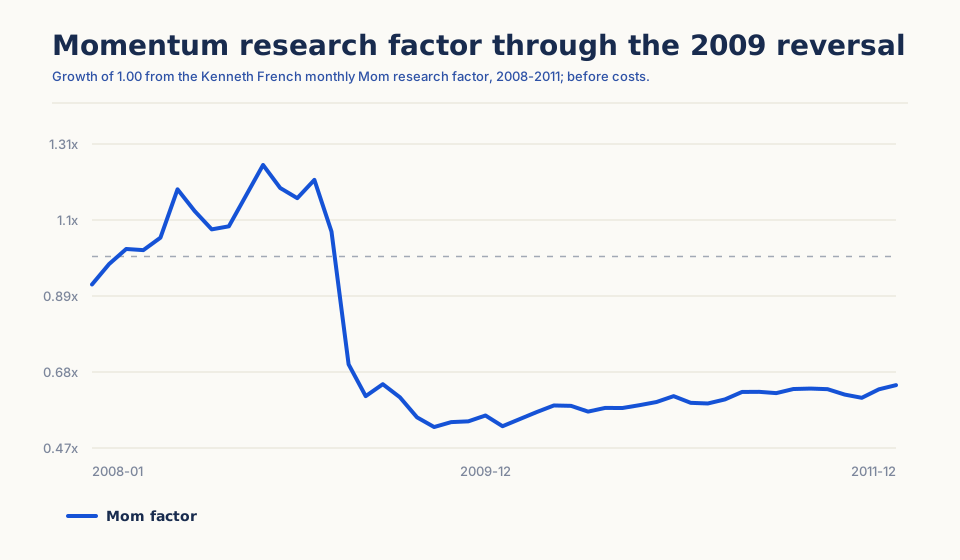
This interval was selected to make a known failure mode visible, not to estimate a typical loss. It connects the earlier explanation—recent losers can rebound together while recent winners lag—with an observed factor path. It does not recreate constituent formation, short availability, fills, or an executable Arizmic strategy.
Further reading
- Kenneth French, Momentum Factor (Mom) definition — Defines the published winner-minus-loser construction; the monthly momentum archive is the retained input for the selected 2008–2011 chart. The series is a research factor, not an executable portfolio return.
- Jegadeesh and Titman, “Returns to Buying Winners and Selling Losers” (1993) — Establishes the canonical US equity winner-minus-loser result and explicitly varies formation and holding periods, making clear that “momentum” is a family of designs.
- Daniel and Moskowitz, “Momentum Crashes” (2016) — Documents momentum’s conditional crash behavior, particularly after market declines followed by sharp rebounds, and supplies the mechanism examined in the selected case.
- Asness, Moskowitz, and Pedersen, “Value and Momentum Everywhere” (2013) — Extends relative momentum and value constructions across asset classes and studies their interaction; it supports broader comparison without making every market implementation interchangeable.