Momentum asks whether movement tends to continue
Momentum is the idea that a market which has moved in one direction may be more likely to keep moving in that direction for a while. It does not mean that every rising market will rise tomorrow, or that prices possess a permanent “force.” It is a statistical hypothesis about conditional returns: after a defined past move, does the distribution of later returns differ from its ordinary distribution?
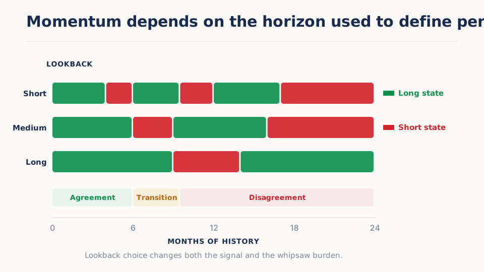
The horizon is part of the definition. A futures contract can be up over twelve months, down over ten days, and rising during the current session. Those are not contradictory observations. They are three different signals built from three different histories.
Momentum also differs from trend in a useful way. Momentum usually measures past change, such as a trailing return. Trend is the broader strategy family that turns evidence of persistence into positions; moving-average filters and breakout rules can be trend rules without directly using a trailing-return signal.
Finally, time-series and cross-sectional momentum answer different questions:
- Time-series momentum compares one market with its own history. “Has this future risen over the last six months?”
- Cross-sectional momentum compares peers at one point in time. “Which stocks rose the most relative to the rest of this universe?”
This guide develops the first question. Cross-sectional construction has its own guide because ranking, neutrality, and portfolio formation create different risks.
Why persistence might exist
Several mechanisms could produce a period of continuation.
Information may reach investors at different times, and some institutions may need days or months to move large portfolios. Investors can also underreact to new information, anchor on earlier beliefs, or follow an emerging move only after it becomes visible. In futures, slowly changing macroeconomic conditions and hedging demand can sustain direction across related markets.
A trend strategy can also be understood through its payoff shape. It accepts many small reversals and missed starts in exchange for remaining exposed during the occasional extended move. This does not require every trend to be caused by one behavioral bias. It does require the large moves to survive the strategy’s lag, turnover, and losses in directionless periods.
Cross-asset futures research documents declared time-series-momentum constructions across multiple markets. That evidence supports investigating persistence; it does not identify one universal cause or validate an arbitrary lookback.
Those explanations are hypotheses, not licenses to choose any lookback that performed well. If the effect disappears with a one-period decision lag or after costs, the appealing story does not rescue the rule.
The decisions hidden inside a simple momentum rule
| Decision | Examples | What it changes |
|---|---|---|
| Measurement | Trailing return, return excluding the latest month, filtered slope | Which part of the past counts as persistence |
| Lookback | Days, weeks, or months | The economic horizon and reaction speed |
| State | Positive/negative, threshold band, or ranked strength | How easily the rule changes direction |
| Exposure | Long/flat or long/short | Market beta, shorting assumptions, and tail behavior |
| Evaluation | Every bar, daily, weekly, or monthly | Turnover and the earliest valid decision |
| Sizing | Fixed units, fixed notional, or volatility target | Which markets and periods dominate risk |
| Exit | Signal reversal, timeout, stop, or a separate risk rule | Whether the strategy can retain extended winners |
A rule is not reproducible until each decision has an answer. “Buy positive momentum” leaves open both the information used and the trade that follows.
A complete rule walkthrough
Consider an illustrative weekly time-series rule:
- After Friday’s bar has completed, calculate the contract’s total return over the previous 26 completed weeks.
- If the return is above +2%, label the next state long. If it is below −2%, label it short. Inside that neutral band, retain no position.
- Submit any position change at the next eligible modeled event. The Friday close that completed the signal cannot also be assumed as an earlier fill.
- Set exposure so that a declared volatility estimate contributes a target amount of risk, subject to a leverage limit.
- Re-evaluate after each completed Friday. A separate protective exit may reduce risk sooner, but it must be specified before the study.
Illustrative example. Suppose the 26-week return is +8%, the next state is long, and the volatility rule assigns 0.7 units. That is the entire implication of the signal. It does not say the following week will be positive; it says the strategy accepts the long distribution associated with that predeclared state.
The neutral band is not a free improvement. It may reduce whipsaws, but it can also delay re-entry after a genuine reversal. Volatility scaling is similarly not just housekeeping: it changes exposures through time and can create much of the apparent consistency in a multi-market result.
How to design an informative study
Start with a baseline a reader can reason about:
- one liquid market or a predeclared cross-asset universe;
- one trailing-return definition;
- one evaluation schedule;
- long/flat and long/short reported separately;
- fixed exposure shown beside risk-scaled exposure; and
- costs linked to actual changes in position.
Then test a small, ordered neighborhood of horizons, such as 13, 26, and 52 weeks. The point is not to select the tallest result. It is to learn whether slower or faster persistence produces a coherent change in turnover, lag, and drawdown.
Useful diagnostics include:
- percent of time long, short, and neutral;
- number of state changes and cost per change;
- return contribution by instrument and calendar period;
- performance during rising and falling volatility;
- average loss during whipsaw sequences;
- contribution from the largest five trends; and
- behavior after adding one decision-period of delay.
The experiment should preserve failed transitions. Removing “obvious” false signals after seeing them changes the research question.
What would count as credible evidence
A positive backtest is only the first observation. Confidence rises when the rule survives nearby lookbacks, reasonable timing and cost assumptions, different liquid markets, and periods not used to choose its design.
The economic interpretation matters too. A broad futures program and a single-stock long-only rule can both be called momentum while carrying very different exposures. Report the long and short legs, asset groups, market beta, and volatility scaling separately enough to show what generated the result.
Evidence weakens when one instrument or crisis produces most of the profit, when performance exists only at one finely selected horizon, or when continuous futures construction and roll treatment determine the result.
Where momentum fails
- Whipsaw: repeated reversals produce small losses and high turnover before a sustained move appears.
- Crowded reversal: markets that moved together can reverse together, creating correlated losses across an apparently broad universe.
- Late entry: a slow lookback can identify a trend only after much of the move has occurred.
- Risk-scaling lag: exposure may be cut after a volatility shock and rebuilt during the next quiet period, changing the intended bet.
- Construction error: stale prices, incorrect contract rolls, or a survivorship-biased universe can manufacture persistence.
- Narrative leakage: choosing the horizon after inspecting the chart turns a test into an explanation of known history.
Momentum is therefore not “buy what went up.” It is a family of timing, exposure, and risk decisions built around a falsifiable persistence hypothesis.
Try it in Arizmic
Strategy composition
Build the premise with shipped signals
Express persistence as a completed-bar directional state, require a separate measure of trend quality, and control exposure when volatility changes. The recipes below test the same momentum premise with either return direction or a crossover event.
These are starting structures, not presets or evidence of an edge. Choose one, replace the bracketed decisions, and keep the signal roles separate as you test it.
Composition 01
Own-return direction with strength and volatility control
Return-state recipe- ROCDirectional state
- ADX/DMITrend-quality gate
- EWMA VolatilityExposure scaler
Data: OHLCV Bars
View configuration and complete ruleHide recipe details
Composition 01
Own-return direction with strength and volatility control
ROC
Directional state
Rate of Change supplies the strategy’s simplest claim: price is above or below where it stood at the chosen horizon.
Configure
- window · [momentum lookback]
- Set this to the horizon over which persistence is being claimed.
Use the output
- roc
- Allow long exposure when ROC is above [long threshold] and short or flat exposure when it is below [short threshold].
ADX/DMI
Trend-quality gate
ADX separates directional persistence from a weak, range-like state; the DMI outputs can also prevent the strength reading from being mistaken for direction.
Configure
- window · [strength lookback]
- Choose a horizon that measures the trend state without duplicating the ROC endpoint exactly.
Use the output
- adx
- Permit a new position only when ADX is at or above [minimum strength].
- plus_di
- For a long, require +DI to be above -DI at the decision bar.
- minus_di
- For a short, require -DI to be above +DI at the decision bar.
EWMA Volatility
Exposure scaler
EWMA Volatility lets the same directional rule target more comparable risk as recent variability changes.
Configure
- lambda · [decay factor]
- Control how quickly the risk estimate reacts to new returns.
- return_kind · [simple or log return]
- Match the return definition used by the rest of the strategy.
- annualization_bars · [bars per year]
- Match the declared bar interval instead of assuming a daily convention.
- zscore_window · [volatility context window]
- Use only if the recipe also compares current volatility with its own recent history.
Use the output
- ewma_volatility
- Scale target exposure toward [risk target] divided by the reported volatility, subject to [maximum leverage].
Assemble the rule
- Entry
- After a completed bar, enter in the ROC direction only when ADX and the matching DMI direction pass their gates.
- Exit
- Exit when ROC loses the directional threshold, the matching DMI direction reverses, or [maximum holding/invalidation rule] is reached.
- Decision time
- Read all three signals from the completed decision bar and make the earliest permitted order decision on the next event.
- Sizing
- Use inverse EWMA-volatility sizing with an explicit exposure cap; do not let the scaler create direction.
Useful variations
- Compare long/flat with symmetric long/short exposure while leaving every other rule unchanged.
- Test a small neighborhood of ROC and ADX windows rather than selecting one isolated pair.
- Replace the ADX gate with no strength gate to measure whether it adds information or merely reduces trade count.
Keep in view
ADX can stay elevated after a trend has begun to reverse, while volatility scaling can increase exposure after a quiet period just before a break. Both controls need independent caps and failure analysis.
Composition 02
Crossover event with regime and ATR guardrails
Transition-event recipe- Moving-Average CrossEntry transition
- Trend RegimeEligibility state
- Wilder ATRRisk distance
Data: OHLCV Bars
View configuration and complete ruleHide recipe details
Composition 02
Crossover event with regime and ATR guardrails
Moving-Average Cross
Entry transition
The crossover outputs turn a persistent moving-average relationship into a one-bar transition event.
Configure
- fast_window · [fast window]
- Set the response speed of the leading average.
- slow_window · [slow window]
- Set the broader trend reference and keep it longer than the fast window.
Use the output
- cross_up
- Use a true event as the long-entry trigger after the decision bar completes.
- cross_down
- Use a true event as the short-entry trigger or long exit, according to the declared exposure policy.
- spread
- Require the spread to remain beyond [buffer] if the design uses confirmation rather than a raw cross.
Trend Regime
Eligibility state
Trend Regime combines strength, slope, and spread thresholds into a categorical guard so a crossover need not trade every range-bound transition.
Configure
- adx_threshold · [minimum strength]
- Define the directional-strength component of eligibility.
- slope_threshold · [minimum slope]
- Require a meaningful trend slope instead of a nearly flat crossover.
- spread_threshold · [minimum spread]
- Reject transitions whose moving-average separation is too small.
Use the output
- trend_regime
- Permit the crossover only in [eligible trend-regime state or states].
Wilder ATR
Risk distance
Wilder ATR converts current bar-scale variability into a consistent stop or position-risk distance.
Configure
- window · [ATR window]
- Match the risk estimate to the expected holding horizon without copying the slow trend window.
Use the output
- atr
- Set the initial risk distance to [ATR multiple] times ATR and derive size from the declared risk budget.
Assemble the rule
- Entry
- Enter only when a fresh cross event and an eligible Trend Regime are both known on the completed bar.
- Exit
- Exit on the opposite cross, an adverse regime change, or the declared ATR-based protection rule.
- Decision time
- A cross is not known before the bar closes; place the decision on the next eligible event and keep the fill assumption explicit.
- Sizing
- Translate the ATR risk distance into units under [risk per position] and [maximum gross exposure].
Useful variations
- Compare a fresh crossover trigger with persistent spread-above-zero state.
- Add one-bar or multi-bar confirmation without moving the historical entry timestamp backward.
- Remove Trend Regime while keeping the same crosses to isolate whether the gate helps.
Keep in view
A regime gate built from related trend inputs can simply restate the crossover in a more complicated form. Inspect incremental selectivity and whipsaw reduction rather than assuming three signals mean three independent confirmations.
Ask the AI Companion
Draft this strategy
Turn the guide’s momentum idea into a simple draft and explain the main choices before asking you to configure them.
I want to create a trend-following strategy for [instrument] that detects sustained directional moves and seeks to profit by remaining with them while they persist. Recommend the timeframe and trend horizon you consider the best starting point for this instrument, explain your reasoning, and then build the strategy for me using suitable Arizmic signals or a custom signal if one is needed.
Extend it in Marimo
Begin from a retained Study so every candidate, parameter choice, and reported outcome keeps its provenance.
Compare the two displayed momentum compositions and show exactly when their directional states agree, diverge, or reverse.
- Bring in
- engine-reported ROC, DMI, ADX, crossover, regime, ATR, and volatility outputs, decision timestamps, positions, and fills, turnover, costs, and retained candidate identifiers
- Build
- multi-horizon state and transition timeline, agreement matrix with forward paths aligned from the original decision time, net outcome and whipsaw table partitioned by trend and reversal states
Interpretation: A useful composition should remain understandable when the signals disagree. If results improve only in the one parameter pair chosen after inspection, treat that as selection rather than broad persistence.
Value origin: Signal values, decisions, fills, costs, and retained metrics are engine-reported. Agreement labels, state partitions, and any custom forward-path summaries are notebook-derived and must retain the original timestamps.
With Companion: Ask Companion to draft the comparison cells against the retained Study, preview the diff, inspect the typed reads and timestamp alignment, then apply it explicitly.
Further reading
- Moskowitz, Ooi, and Pedersen, “Time Series Momentum” (2012) — Defines and tests own-history momentum across 58 liquid futures and forward contracts. Its pooled, volatility-scaled construction is the literature’s starting point, not evidence for every lookback, market, or sizing rule.
- Hong and Stein, “A Unified Theory of Underreaction, Momentum Trading, and Overreaction in Asset Markets” (1999) — Models how gradual information diffusion can create short-run underreaction and how momentum trading may contribute to later overreaction. It offers a plausible mechanism, not proof that the mechanism drives a particular trend.
- Kim, Tse, and Wald, “Time Series Momentum and Volatility Scaling” (2016) — Re-examines 55 futures contracts and finds that volatility scaling drives much of the reported alpha. It helps separate the momentum signal from sizing, leverage, and benchmark effects.
- Goyal and Jegadeesh, “Cross-Sectional and Time-Series Tests of Return Predictability: What Is the Difference?” (2018) — Shows why time-series and cross-sectional momentum tests are not interchangeable and identifies time-varying net-long exposure as an important contributor to time-series strategy results.
- Huang, Li, Wang, and Zhou, “Time Series Momentum: Is It There?” (2020) — Finds weak asset-level and out-of-sample evidence that the standard 12-month return predicts the following month, despite profitable strategy returns. It makes the crucial distinction between forecastability and portfolio payoff.
- Hurst, Ooi, and Pedersen, “A Century of Evidence on Trend-Following Investing” (2017) — Extends a specified diversified trend simulation across global markets using reconstructed data back to 1880. It adds historical breadth, but represents hypothetical strategy performance under declared assumptions.