Risk is not one number
Volatility, drawdown, and tail risk describe different ways a strategy can hurt its owner.
Volatility describes how widely returns vary around their average. It is a measure of typical dispersion. Drawdown describes the fall from a previous equity peak and therefore depends on the order of returns. Tail risk describes unusually severe outcomes that ordinary variation may understate.
A strategy can look mild under one lens and dangerous under another. A short-volatility strategy may report many small, stable gains and only occasional large losses. Its ordinary volatility can look attractive before the tail event arrives. A volatile trend strategy may fluctuate often but cap losses during the particular crisis that harms the first strategy. Neither label alone tells the whole story.
| Risk lens | What it preserves | What it can miss |
|---|---|---|
| Volatility | Typical dispersion at a declared frequency | Direction, path order, and losses absent from the sample |
| Drawdown | The path from each running peak through loss and recovery | The probability of a worse future path |
| Tail measure | Severity or frequency beyond a chosen threshold | Events outside the data or distributional assumptions |
The measures complement one another because they discard different information. None is a complete translation of “how much can I lose?”
Volatility measures ordinary variation
The standard deviation of periodic returns is the most common volatility measure. In plain language, it asks how far returns typically sit from their sample average.
If daily returns are mostly between −0.5% and +0.5%, their volatility will be lower than a series that regularly moves between −2% and +2%. That does not say which series has the higher average return, which one suffers the deeper drawdown, or whether the large observations are gains or losses.
Volatility also depends on frequency. Daily, weekly, and monthly observations are different samples. Converting one to another with a square-root rule assumes a form of independence and stable variance that many strategies do not have. Smoothed prices, overlapping positions, stale marks, and illiquid assets can make measured volatility artificially low.
Drawdown measures damage along the path
Drawdown compares current equity with the highest equity previously reached:
Here, is equity at time . Drawdown is zero at a new high and negative below that high. Maximum drawdown is the most negative observed value. Some reports display the same loss as a positive magnitude. Under the signed convention above, a fall from 120 to 90 is −25%; under a magnitude convention, it is reported as 25%. The sign convention must be known before comparing two systems.
Illustrative example. Suppose equity rises from 100 to 120, then falls to 90. The loss from the original 100 is 10%, but the drawdown from the 120 peak is 25%. A result that calculates loss only from starting capital would miss the experience of losing one quarter of the peak account value.
Drawdown is path-dependent. Two strategies can have the same ending return and the same set of monthly returns in a different order, yet produce different peak losses, recovery times, and margin pressure.
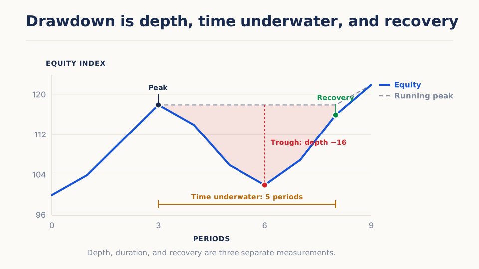
Depth, duration, and recovery are separate
Maximum drawdown reports the deepest historical decline, but not how long the strategy remained below its high or how often similar declines occurred.
- Drawdown depth is the percentage loss from peak.
- Duration is the time spent below the prior peak.
- Recovery time is the time required to regain that peak.
- Underwater frequency describes how often the strategy is in drawdown.
A quick 20% fall and recovery may be easier to finance than a 10% decline that persists for three years. Both deserve more context than one maximum statistic.
Tail risk asks about unusually bad outcomes
Return distributions often contain more extreme observations than a normal curve would suggest. Averages and standard deviations can understate this when losses are asymmetric, clustered, or produced by a strategy that sells insurance-like exposure.
Value at Risk estimates a loss threshold at a chosen probability and horizon. Expected Shortfall, also called Conditional Value at Risk in many contexts, asks about the average loss beyond that threshold. These numbers depend on the distribution or resampling method used, the sample window, and whether dependence is preserved.
For example, saying “the 95% one-day loss threshold is 2%” does not describe how bad the remaining 5% can be. Expected Shortfall tries to summarize that remaining tail, but a historical estimate cannot include events absent from the sample.
A three-strategy comparison
Imagine three illustrative return paths:
| Strategy | Typical months | Rare behavior | Main risk lens |
|---|---|---|---|
| A | Small gains and losses | Occasional sharp loss | Tail loss and skew |
| B | Frequent wider swings | Losses recover quickly | Volatility and sizing |
| C | Quiet marked returns | Sudden repricing after stale periods | Data quality and hidden volatility |
Strategy A may show attractive ordinary volatility until a tail loss occurs. Strategy B may have the highest volatility but manageable drawdown under smaller sizing. Strategy C may appear safest because its prices update slowly, even though executable risk is accumulating.
The research decision is not to pick a favorite metric. It is to identify which loss process the strategy can produce and whether the data makes that process visible.
Stress the assumption behind the statistic
Ask how the risk picture changes when:
- returns are evaluated at a different but defensible frequency;
- costs rise during volatile or illiquid periods;
- correlated positions lose together;
- the largest historical loss is repeated or exceeded;
- stale marks are replaced with executable prices;
- position scaling reacts with a delay;
- the sample begins or ends in a different regime.
The purpose is not to invent a precise disaster forecast. It is to expose which conclusion relies on calm variation, easy liquidity, or one favorable path.
Common risk-reading mistakes
- Calling low volatility low risk without examining skew and tails.
- Reporting drawdown from starting capital instead of the running peak.
- Comparing annualized volatility from incompatible frequencies.
- Treating the worst historical loss as a hard upper bound.
- Ignoring drawdown duration and the capital required to survive it.
- Estimating risk from smoothed or stale prices.
- Reducing exposure after volatility rises without accounting for the cost and timing of that rebalance.
Further reading
- Fama, “The Behavior of Stock-Market Prices” (1965) — Seminal empirical evidence that stock-price changes exhibit distributional behavior that a simple normal model does not fully capture.
- Chekhlov, Uryasev, and Zabarankin, “Drawdown Measure in Portfolio Optimization” (2005) — Treats drawdown as a path-dependent object and distinguishes maximum, average, and conditional drawdown measures.
- Rockafellar and Uryasev, “Optimization of Conditional Value-at-Risk” (2000) — Formalizes expected loss beyond a selected tail threshold and clarifies why it contains information that a loss quantile alone does not.
- Lo, “The Statistics of Sharpe Ratios” (2002) — Shows why serial dependence changes volatility scaling and invalidates automatic square-root-of-time translation in the general case.