Diversification means losses do not all arrive for the same reason
Diversification is the reduction in portfolio dependence that comes from combining genuinely different sources of return. Holding more positions is not enough. Twenty technology stocks, five equity-index strategies, or three trend rules using different lookbacks can still be one concentrated bet.
Correlation is one way to summarize how two return series moved together in a sample. A value near +1 means they tended to be above or below their averages together. A value near −1 means they tended to move in opposite directions. A value near zero means little linear co-movement at that frequency in that sample.
Correlation is useful because portfolio risk depends on interaction, not just the volatility of each component. It is incomplete because dependence can be nonlinear, unstable, and strongest during the losses that matter most.
A simple two-strategy example
Illustrative example. Imagine equally weighted pairs of strategies. Every strategy has 10% volatility at the same chosen frequency.
- Strategy A and Strategy B have correlation +0.9. They usually gain and lose together. Combining them mostly divides capital between similar paths.
- Strategy A and Strategy C have correlation 0.0. Their ordinary monthly moves do not line up consistently. The combination may have a smoother path.
- Strategy A and Strategy D have correlation −0.5. D often gains when A loses, offering stronger historical offset.
The result is not guaranteed. Correlation is estimated with error, and D’s negative relationship might disappear in a new regime. The example shows why the same component volatilities can produce different portfolio volatility.
For two positions with weights and , volatilities and , and correlation , portfolio variance includes a covariance term:
The final term is where interaction enters. Lower correlation can reduce variance, but only under the estimated relationship and chosen weights.
With two 50% weights and 10% component volatility, the formula gives:
| Pair correlation | Portfolio volatility |
|---|---|
| +0.9 | About 9.75% |
| 0.0 | About 7.07% |
| −0.5 | 5.00% |
The low-correlation pair is not safer because either component changed. It is safer in this calculation because their deviations do not arrive together as often. Change the weights, volatilities, or correlation estimate and the answer changes.
Frequency and alignment change the number
Daily correlation and monthly correlation can differ because positions overlap, markets close at different times, and effects operate at different horizons. Price levels that trend upward together can show high correlation even when their returns provide little information about one another. Portfolio research normally compares aligned returns, not raw price levels.
Missing dates create another trap. Pairwise deletion can estimate each correlation from a different sample. Forward-filled prices can manufacture zero returns. Asynchronous closing times can make related markets appear weakly correlated because the same information enters on different rows.
State the return frequency, common calendar, missing-data rule, currency, and sample window before interpreting the matrix.
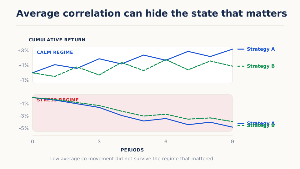
Average correlation can hide crisis dependence
Suppose a carry strategy and an equity strategy have low full-sample correlation. Both may still depend on liquid funding and lose during a sudden deleveraging. Their calm-period independence is real, but it is not protection in the state that threatens the portfolio.
Useful extensions include:
- rolling correlation to show change, while recognizing the estimate is noisy;
- downside or tail co-movement during large losses;
- drawdown overlap and simultaneous loss frequency;
- common factor, instrument, direction, and liquidity exposure;
- scenario-based questions about what could force both positions to unwind.
The goal is not to find the most sophisticated coefficient. It is to identify whether supposedly different strategies can fail together.
Strategy overlap exists before return correlation
Two return streams can have low historical correlation and still share a fragile mechanism:
- both trade the same instruments at the same time;
- both rely on the same volatility estimate or regime filter;
- both enter after similar price moves under different names;
- both require liquidity during a reversal;
- both were selected from the same historical episode.
Position overlap, signal overlap, turnover overlap, and capacity overlap can be visible before enough returns exist to estimate the risk reliably. Those diagnostics are especially important for new strategies.
Diversification can dilute rather than improve
A low-correlation component is not automatically worth owning. If it has a negative expected return after costs, unreliable data, or tiny capacity, adding it may reduce measured volatility while worsening the portfolio’s purpose.
Evaluate the component on its own merits, then evaluate its marginal contribution to the existing portfolio. Ask whether it improves return, reduces drawdown, changes tail behavior, or supplies exposure in a state the portfolio currently lacks.
A practical diversification review
- Align net return series on one calendar and currency basis.
- Inspect full-sample and rolling correlation.
- Compare correlation during the largest portfolio and component drawdowns.
- Map common instruments, factors, signal families, and liquidity needs.
- Recalculate risk after plausible correlation increases.
- Examine marginal contribution under the proposed weights.
- Prefer broad stable neighborhoods to one optimized covariance estimate.
Common mistakes
- Calling a large position count diversified.
- Calculating correlation on price levels.
- Treating one full-sample matrix as permanent.
- Ignoring time-zone and missing-date alignment.
- Selecting a component solely for low historical correlation.
- Optimizing weights against a noisy matrix without constraints or stress.
- Forgetting that shared liquidity and leverage can create dependence absent from ordinary returns.
Further reading
- Markowitz, “Portfolio Selection” (1952) — Establishes how individual variances and pairwise covariances combine into portfolio risk.
- Engle, “Dynamic Conditional Correlation” (2002) — Provides a parsimonious framework in which conditional correlations can change rather than remaining fixed through the sample.
- Longin and Solnik, “Extreme Correlation of International Equity Markets” (2001) — Finds that dependence among major equity markets behaves asymmetrically in extreme returns, with stronger correlation in bear markets than an unconditional estimate suggests.
- DeMiguel, Garlappi, and Uppal, “Optimal Versus Naive Diversification” (2009) — Shows how parameter-estimation error and turnover can erase the theoretical advantage of optimized weights over a simple equal-weight baseline.