Combining strategies means deciding how they share one portfolio
A multi-strategy portfolio runs more than one return process under a common capital and risk budget. The aim is often diversification: a loss in one strategy may be offset or avoided by another that responds differently.
Different names do not guarantee different risk. A momentum strategy and a breakout strategy can both buy the same futures during the same trend. A VWAP reversion strategy and an opening-range fade can both become short the same instrument during a strong upward repricing. Their logic is different, but the portfolio experiences the combined position and combined loss.
Combining strategies therefore requires more than a correlation matrix. The researcher must inspect positions, instruments, timing, return dependence, drawdown overlap, capacity, and competition for capital.
Diversification has several layers
| Layer | Question | Example of hidden overlap |
|---|---|---|
| Position | Are strategies long or short the same instrument together? | Two trend rules both long an index future |
| Exposure | Do different holdings share a factor or macro risk? | Equity value and credit both exposed to growth stress |
| Return | Do net returns move together in ordinary periods? | Similar daily P&L despite different trades |
| Drawdown | Do losses begin, deepen, and recover together? | Reversion sleeves all fail during repricing |
| Tail | Do correlations rise specifically during large losses? | Distinct markets sell off under one liquidity shock |
| Capacity | Do strategies demand the same liquidity at the same time? | Several exits hit one thin close |
| Capital | Can simultaneous signals all be admitted? | Independent backtests each assume the full account |
A low full-sample correlation can coexist with severe tail co-loss. The period when diversification is most needed deserves its own analysis.
Why combining can help
If strategies respond to genuinely different mechanisms and states, their idiosyncratic outcomes may partially offset. A slow trend sleeve, a market-neutral relative-value sleeve, and an intraday strategy can have different clocks, holdings, and failure modes.
Diversification cannot turn a weak or untradeable strategy into a strong one. Adding a negatively correlated stream with negative expected net return may smooth history while destroying capital. Each component should first have a clear role and defensible standalone evidence.
The combination also creates behavior that standalone backtests cannot show: orders compete for cash, one strategy may block another under exposure limits, positions can net, and portfolio halts can change later trades.
Put components on a comparable basis
Before allocating, align:
- date range, timezone, and session treatment;
- return definition and starting capital;
- fees, spread, impact, and financing;
- execution fidelity;
- mark-to-market and missing-data policy;
- risk measure and evaluation frequency; and
- treatment of inactive periods.
A daily-return strategy and an intraday trade list cannot simply be placed in adjacent spreadsheet columns and correlated without resolving their common clock and equity accounting.
An illustrative two-strategy portfolio
Illustrative example. Suppose Strategy A and Strategy B each have a standalone risk target of 10 units. On a given day:
- A requests a +6-unit long position in an index future.
- B requests a −4-unit short position in the same future.
- the portfolio has a maximum gross open risk of 12 units and an instrument limit of 8.
At the account level, the requests can net to +2 units if the execution and policy permit. But gross demand was 10 units, and both strategies still have distinct ownership of their trades and P&L. If B’s short is rejected or delayed, the portfolio is not hedged as the standalone return series implied.
Now assume both strategies request +6. Their standalone backtests each fit a 10-unit budget, but together they breach the instrument limit. Priority, clipping, or rejection changes which return stream actually occurs.
This is why a portfolio simulation must evaluate shared capital and admission, not merely add historical curves.
Designing the combination study
Start with transparent baselines:
- Each strategy alone under the common economics.
- Equal capital across strategies.
- Equal standalone risk under explicit caps.
- The proposed allocation and admission policy.
Add strategies one at a time. For each addition, measure:
- change in net return and drawdown;
- marginal and total volatility;
- position and instrument overlap;
- ordinary and downside correlation;
- simultaneous drawdown duration;
- strategy contribution and concentration;
- rejected or clipped opportunities;
- netted versus synchronized turnover; and
- combined capacity and impact.
Use rolling and stressed windows descriptively, but do not optimize a new set of weights for every historical window and call the result stable.
Correlation is a summary, not the decision
Correlation measures linear co-movement under a chosen sample. It can be noisy when histories are short, misleading when return distributions are nonlinear, and unstable across states.
Add drawdown-overlap tables, conditional correlations during portfolio losses, and holdings-based diagnostics. Look at the actual dates of the worst combined outcomes. The objective is to understand shared causes, not to invent a new story for each loss.
Important failure modes
- Different backtest clocks or pricing rules make streams incomparable.
- Full-sample correlation hides common tail losses.
- One sleeve dominates portfolio risk despite equal capital.
- Standalone simulations each assume capital that cannot be used twice.
- Netting reduces ordinary turnover but synchronized exits raise impact.
- Optimized weights exploit covariance noise.
- A portfolio halt or risk limit changes the opportunity set in ways a summed curve cannot represent.
Real-world case
Historical case. Published US HML value and Mom momentum research series provide a reproducible illustration of differently behaving factors. For each month from January 2000 through December 2019, an illustrative blend allocates half to the published HML return and half to the published Mom return, then compounds the blended monthly result.
Over that selected interval, Mom compounded to 1.054, HML to 1.561, and the 50/50 blend to 1.478 before any implementation costs. Their maximum drawdowns were 57.85%, 38.98%, and 33.85%, respectively. The calculation uses retained monthly momentum and five-factor archives with data through May 2026. The blend did not produce the highest ending value; it produced a less severe historical drawdown than either component in this particular window.
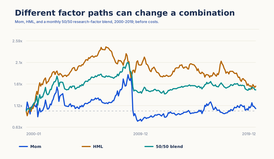
This is not evidence that a fixed 50/50 factor portfolio is optimal. The inputs are long-short research factors, the blend assumes free monthly rebalancing, and the window is selected. It demonstrates the question a combination study should ask: did the components lose at different times strongly enough to change the portfolio path after realistic ownership and costs?
Try it in Arizmic
Portfolio composition
Combine complementary saved strategies
Combine independently saved strategies whose horizons, market behavior, and failure modes may complement one another, then make their overlap, shared capital, and conflict policy explicit. The recipes below illustrate distinct component roles; the Portfolio draft works from matching saved Strategy Configurations rather than merging their signals into one Strategy IR.
The signal recipes illustrate possible component roles. The Portfolio draft works from matching saved strategies and applies explicit allocation, admission, shared-capital, and risk policies.
Composition 01
Trend-or-reversion state router
Conditional-sleeve recipe- Trend RegimeTrend-sleeve eligibility
- Oscillator RegimeReversion-sleeve eligibility
- EWMA VolatilityShared risk budget
Data: OHLCV Bars
View configuration and complete ruleHide recipe details
Composition 01
Trend-or-reversion state router
Trend Regime
Trend-sleeve eligibility
Trend Regime identifies the states in which the trend component is allowed to act.
Configure
- adx_threshold · [strength threshold]
- Define trend eligibility.
- slope_threshold · [slope threshold]
- Require directional slope.
- spread_threshold · [spread threshold]
- Require meaningful separation.
Use the output
- trend_regime
- Enable the trend component only in [declared state].
Oscillator Regime
Reversion-sleeve eligibility
Oscillator Regime provides a standardized displacement state for the reversion component.
Configure
- window · [oscillator window]
- Define the local anchor history.
- lower_threshold · [lower threshold]
- Define long-reversion candidates.
- upper_threshold · [upper threshold]
- Define short-reversion candidates.
Use the output
- regime
- Enable reversion only in [declared non-trend state and extreme].
EWMA Volatility
Shared risk budget
EWMA Volatility puts both components under one capped risk convention instead of letting the more volatile sleeve dominate.
Configure
- lambda · [decay factor]
- Set risk responsiveness.
- return_kind · [return definition]
- Match strategy returns.
- annualization_bars · [bars per year]
- Match the interval.
- zscore_window · [context window]
- Use only for declared volatility-state diagnostics.
Use the output
- ewma_volatility
- Scale the active component toward [shared risk target] under [gross cap].
Assemble the rule
- Entry
- Route a completed-bar decision to the trend or reversion component according to mutually exclusive state rules; define what happens when neither or both qualify.
- Exit
- Use each component’s own exit, plus a shared gross-risk and state-transition policy.
- Decision time
- Evaluate routing and component signals on the same completed decision bar before the next-event order decision.
- Sizing
- Allocate the shared risk target to the active component, with explicit handling if both are allowed.
Useful variations
- Compare hard routing with a version that allows both components at reduced risk.
- Use equal risk per component versus state-dependent risk.
- Report results for each sleeve, routing state, and combined path.
Keep in view
Trend and oscillator states are derived from the same price series. Routing can reduce direct rule conflict, but it does not create independent return sources.
Composition 02
Trend transition plus VWAP displacement under volatility policy
Dual-premise recipe- Moving-Average CrossTrend component
- Session VWAP DistanceIntraday reversion component
- Volatility RegimeConflict and risk policy
Data: OHLCV Bars
View configuration and complete ruleHide recipe details
Composition 02
Trend transition plus VWAP displacement under volatility policy
Moving-Average Cross
Trend component
Moving-Average Cross supplies a directional transition and persistent spread state.
Configure
- fast_window · [fast window]
- Set trend responsiveness.
- slow_window · [slow window]
- Set the broader trend reference.
Use the output
- cross_up
- Create the trend long candidate.
- cross_down
- Create the trend short candidate or exit.
- spread
- Retain persistent trend state.
Session VWAP Distance
Intraday reversion component
Session VWAP Distance supplies a separate intraday displacement premise.
Configure
- zscore_window · [distance history]
- Normalize distance within the intended session context.
Use the output
- zscore
- Create the reversion candidate beyond [thresholds].
Volatility Regime
Conflict and risk policy
Volatility Regime can determine whether one component is blocked, reduced, or merely labeled during unstable conditions.
Configure
- high_z_threshold · [high threshold]
- Define the high-risk state.
- low_z_threshold · [low threshold]
- Define the quiet state.
Use the output
- volatility_regime
- Apply [component-specific policy] without using regime as direction.
Assemble the rule
- Entry
- Apply declared precedence when trend and reversion candidates conflict; otherwise enter the qualifying component after bar completion.
- Exit
- Use component-specific exits and a shared conflict, gross exposure, and session policy.
- Decision time
- Align both components to the same decision clock and document session resets for VWAP.
- Sizing
- Use [equal risk, capped sleeve budgets, or declared weighting] with total gross and net caps.
Useful variations
- Compare independent sleeve execution with conflict-netted execution.
- Measure overlap in positions, drawdowns, and market states.
- Replace volatility gating with constant component caps to isolate the policy.
Keep in view
Two different signal names can still produce the same directional exposure. Inspect position overlap and loss overlap rather than relying on labels such as trend and reversion.
Ask the AI Companion
Draft this portfolio
Identify complementary strategy roles, explain their likely overlap, and assemble matching saved strategies into a shared-capital Portfolio draft.
I want to build a portfolio-level strategy for [market or instrument]. Suggest a small group of strategies that could complement one another by responding to different market conditions or time horizons—for example, combining short-term mean reversion with longer-term momentum. Explain what each strategy would contribute, where their exposures could still overlap, and which combination you recommend. Then use the matching saved strategies in my library to build a simple starting portfolio with a sensible allocation, clear handling when strategies compete for the same trade or capital, and shared risk limits.
Extend it in Marimo
Begin from a retained Study containing component and combined candidates so the composition can be decomposed.
Show whether the combined path improves because components offset or merely because exposure, timing, or risk changed.
- Bring in
- engine-reported Trend Regime trend_regime, Oscillator Regime regime, EWMA Volatility ewma_volatility, routing states, positions, decisions, fills, costs, and outcomes, component and shared sizing rules, retained candidate and component identifiers
- Build
- component and combined exposure/wealth paths, position, return, and drawdown-overlap matrix, state-routed contribution and conflict-reconciliation table
Interpretation: Focus on the worst joint periods. If components lose together or one dominates risk, the combined label overstates diversification.
Value origin: Signals, positions, decisions, fills, costs, and retained results are engine-reported. Overlap labels, contribution decompositions, and custom routed-state summaries are notebook-derived.
With Companion: Ask Companion to draft reviewed overlap and contribution cells, inspect component alignment and risk normalization, then explicitly apply the diff.
Further reading
- Kenneth French Data Library — Defines and hosts the monthly momentum archive and monthly five-factor archive retained for the selected combination chart. They are reproducible long-short research factors, not executable strategy sleeves with shared capital and costs.
- Markowitz, “Portfolio Selection” (1952) — Establishes how covariance enters portfolio risk and why combining imperfectly related return streams can change the whole portfolio’s variance.
- Engle, “Dynamic Conditional Correlation” (2002) — Provides an estimable model for correlation that changes over time, reinforcing that one full-sample matrix is not a permanent portfolio property.
- Longin and Solnik, “Extreme Correlation of International Equity Markets” (2001) — Uses extreme-value methods to show asymmetric dependence in international equities, with correlation rising in bear markets rather than merely whenever volatility is high.
- DeMiguel, Garlappi, and Uppal, “Optimal Versus Naive Diversification” (2009) — Compares 14 allocation models with a simple 1/N benchmark out of sample, demonstrating why estimated optimal weights need a transparent baseline.