Mean–variance optimization chooses a portfolio from forecasts
Mean–variance optimization asks how to combine assets when a researcher supplies two things:
- an expected return for each asset; and
- a covariance matrix describing how their returns vary together.
The optimizer can seek the lowest modeled variance for a target return, the highest modeled return for a risk limit, or the best trade-off under a chosen risk-aversion parameter. This is the classic mean–variance portfolio-selection problem.
The mathematics can solve the stated problem precisely. The forecasts are the uncertain part. Expected returns are especially noisy, and small input changes can produce very different “optimal” weights. Estimation error can therefore make optimized portfolios unstable and unintuitive.
What covariance contributes
Portfolio risk is not the weighted average of standalone volatilities. If two assets tend to move in opposite directions, their combination can be less variable than either risk estimate alone suggests. The covariance matrix captures those interactions.
With many assets and a short history, the matrix itself becomes unstable. There are pairwise covariance terms for assets. One hundred assets require 4,950 pairwise relationships before estimating expected returns.
Sampling noise can make apparent diversification opportunities look more precise than they are. Shrinkage, factor models, longer windows, and constraints are ways to trade detail for stability.
Why expected returns create extreme weights
An optimizer is designed to emphasize assets with the most attractive forecast relative to modeled risk. If one estimated mean is slightly larger because of noise, the optimizer may concentrate heavily in it. Shorting and leverage can amplify that response.
This behavior is not the solver malfunctioning. It is the solver faithfully using uncertain inputs as if they were known. Constraints can prevent absurd weights, but the resulting portfolio reflects the guardrails as well as the forecast.
Define the optimization problem
| Component | Choices | Research consequence |
|---|---|---|
| Objective | Minimum variance, target return, utility, maximum Sharpe | Defines what “optimal” means |
| Return estimate | Historical mean, factor model, shrinkage, view | Usually the noisiest input |
| Covariance | Sample, shrunk, factor, robust | Controls modeled diversification |
| Constraints | Long-only, bounds, leverage, sector, turnover | Shapes the feasible portfolio |
| Rebalance | Calendar or trigger | Connects weights to costs |
| Cash/financing | Explicit rates and limits | Determines whether leverage is real |
An efficient frontier is a set of portfolios optimal under one input set. It is not a map of future outcomes.
A two-asset calculation
One useful version of the objective asks for the portfolio with the highest forecast return after charging a penalty for forecast variance:
Here, is the vector of portfolio weights, contains the expected returns, is the covariance matrix, and states how strongly the decision penalizes modeled variance. This is a choice function, not a forecast that the utility value will be earned.
Illustrative example. Consider two fully invested, long-only assets. Asset A has a 6% expected return and 10% volatility. Asset B has an 8% expected return and 15% volatility. Their estimated correlation is 0.2, and the illustrative risk-aversion value is . Solving that declared problem gives:
| Input scenario | Weight in A | Weight in B | Forecast return | Forecast volatility |
|---|---|---|---|---|
| Base inputs | 35.85% | 64.15% | 7.28% | 10.92% |
| B return revised from 8% to 7% | 54.72% | 45.28% | 6.45% | 9.54% |
| Correlation revised from 0.2 to 0.6 | 24.14% | 75.86% | 7.52% | 12.97% |
The one-point return revision moves 18.87 percentage points of capital from B to A. Raising correlation removes diversification, but because B still has the higher return forecast, this particular objective concentrates even more in B while accepting higher modeled volatility. Different constraints or a minimum-variance objective would react differently.
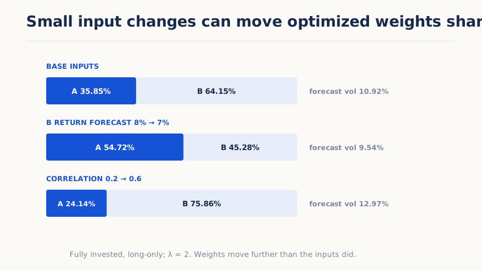
The lesson is not that any row is the right portfolio. It is that input sensitivity, objective choice, and binding constraints belong beside the reported optimum.
A complete research workflow
- Freeze the eligible universe and estimation history before the rebalance.
- Create equal-weight and inverse-volatility baselines.
- Estimate returns and covariance under declared methods.
- Solve the unconstrained problem only as a diagnostic, then apply predeclared practical constraints.
- Record solver status, active constraints, forecast weights, and expected metrics.
- Trade at the next modeled opportunity.
- Compare realized risk, return, turnover, and contribution with the forecasts.
Constraints should not be tuned one by one until historical performance looks reasonable. Their economic purpose—liquidity, concentration, mandate, or turnover—should exist independently.
Stress the inputs, not only the returns
Perturb expected returns, covariance windows, shrinkage strength, and constraint bounds. Plot how weights and forecast risk respond. A broad family of similar portfolios is more credible than a sharp solution that changes completely with minor inputs.
Use rolling out-of-sample re-estimation. At every rebalance, fit only on earlier data, form weights, and evaluate later returns. Include turnover generated by the changing estimates.
Report:
- weight concentration and sign;
- predicted versus realized volatility;
- turnover and costs;
- active constraints;
- sensitivity to inputs;
- contribution by asset and factor; and
- comparison with simple baselines.
Important failure modes
- Sample means dominate weights despite enormous estimation uncertainty.
- Too many assets relative to history destabilize covariance.
- Optimized constraint bounds rescue an in-sample result.
- Solver convergence is mistaken for economic robustness.
- Re-estimation creates costly weight churn.
- Backtests use revised membership or unavailable inputs.
- A single future covariance regime invalidates the historic frontier.
This guide remains conceptual with respect to Arizmic: the standard Portfolio ensemble does not silently supply a mean–variance optimizer. Use it to interpret the method, not as a claim about a hidden product control.
Further reading
- Markowitz, “Portfolio Selection” (1952) — Introduces the mean–variance selection problem and shows how expected returns, variances, and covariances jointly define the efficient set.
- Michaud, “The Markowitz Optimization Enigma: Is ‘Optimized’ Optimal?” (1989) — Explains how estimation error is amplified into unstable, unintuitive weights, directly motivating sensitivity checks and constraints.
- Ledoit and Wolf, “Honey, I Shrunk the Sample Covariance Matrix” (2004) — Develops a practical covariance-shrinkage estimator that trades noisy sample detail for stability; it improves one input rather than eliminating forecast risk.
- DeMiguel, Garlappi, and Uppal, “Optimal Versus Naive Diversification” (2009) — Benchmarks a broad set of estimated allocation rules against 1/N out of sample and quantifies how much history can be needed to overcome estimation error.