Pairs trading bets on a relationship, not two independent prices
Pairs trading combines two related assets into one spread and trades changes in that spread. Instead of predicting that asset A will rise, the strategy asks whether A has become unusually expensive or cheap relative to asset B.
Illustrative example. Imagine two shares exposed to the same industry. If A rises 4% while B is flat, a pairs rule may sell A and buy B. The intended bet is that the gap between them narrows. The trade can lose even if both shares rise: what matters is their relative move after position sizes and costs.
The spread can be a simple difference, a ratio, or a hedged combination such as
where is the estimated amount of B used to offset A. This formula does not make the relationship stable. It only defines the series being tested.
Correlation and cointegration answer different questions
Correlation measures whether changes in two series tend to move together. Two assets can have highly correlated returns while their price levels drift arbitrarily far apart.
Cointegration asks whether a particular combination of nonstationary price series behaves more like a stable, mean-reverting process. It is a stronger and more relevant claim for many pairs strategies, but it is still an estimate from a finite historical sample.
Neither statistic supplies an economic reason for the relationship. Related contracts, share classes, or firms with substitutable businesses may have a defensible link. Two unrelated stocks selected only because a search found a stable past spread are more likely to represent coincidence.
Why relative dislocations might close
Common information may affect related assets at different speeds. Temporary order imbalances, index flows, financing pressure, or local liquidity can move one leg before the other. Arbitrage capital can then help restore the relation.
The counterargument is structural change. An acquisition, index rebalance, contract roll, earnings surprise, capital-structure change, or change in input costs may permanently alter one leg. When that happens, the historic spread is not “more attractive”; it may be measuring a relationship that no longer exists.
Constructing the relationship
| Decision | Examples | Why it matters |
|---|---|---|
| Candidate universe | Economic peers, contract family, or statistical screen | Determines the prior plausibility and search burden |
| Formation period | Fixed historical window or rolling window | Determines which data estimates the relation |
| Spread definition | Difference, ratio, regression residual | Changes the variable expected to revert |
| Hedge ratio | One-for-one, value-neutral, beta-neutral, fitted | Changes directional and factor exposure |
| Normalization | Raw spread, percentage, z-score | Defines an unusual displacement |
| Re-estimation | Frozen per test window or scheduled update | Trades stability against adaptation |
| Break rule | Event flag, parameter drift, timeout, residual behavior | Determines when not to expect convergence |
Selection and trading must be separated. If the same period is used to discover the pair, estimate its hedge, select its threshold, and report performance, the result has no honest holdout.
A two-leg walkthrough
Illustrative example. Assume a formation period ends on June 30. A fitted relation gives , and the spread’s formation mean and standard deviation are 10 and 2.
On July 5:
- A closes at 90;
- B closes at 95;
- the spread is ; and
- the formation-based z-score is .
An illustrative rule sells one unit of A and buys 0.8 units of B at the next eligible modeled event. It exits when the spread reaches a z-score of 0.5, after 20 trading days, or when a relationship-break condition occurs.
If A falls while B falls even more, the spread may widen and the trade loses despite A moving in the expected absolute direction. Both legs, their timing, borrow, financing, and transaction costs belong in the result.
The formation estimates must either remain frozen for the July test or update on a predeclared schedule. Re-estimating after seeing the July path rewrites the trade.
Designing a credible pairs study
Start with economically linked candidates and a transparent selection rule. Compare a fitted spread with a simple ratio or value-neutral baseline. Walk the formation and trading windows forward so every live-style decision uses only earlier data.
Important diagnostics include:
- stability of the hedge ratio across formation windows;
- spread half-life estimates with uncertainty;
- entry count and overlap;
- convergence, timeout, and break-rule rates;
- P&L and cost by leg;
- net factor and market exposure;
- borrow availability and short cost; and
- performance after corporate and index events.
A randomized-pair control from the same point-in-time universe helps reveal how often an apparently attractive spread can be found by search alone. Count every candidate and threshold considered, not just the surviving pair.
What failure looks like
- The estimated relation changes faster than the strategy can adapt.
- A corporate event makes the historical hedge economically meaningless.
- Repeated testing selects a chance relationship with a persuasive chart.
- The spread appears stationary only because the sample is short.
- One leg is difficult or expensive to borrow.
- Bar-level simultaneous fills conceal legging and liquidity risk.
- Historical membership excludes delisted or acquired candidates.
The practical edge, if any, is not “cointegration.” It is a reproducible selection, estimation, execution, and invalidation process whose net relative return survives outside the formation sample.
Real-world case
Historical case. Brent and West Texas Intermediate (WTI) are related crude oil benchmarks, but they are exposed to different delivery locations, transport constraints, inventories, and regional supply shocks. Following military escalation in the Middle East on February 28, 2026, delivery-aligned Brent futures rose faster than WTI as Strait of Hormuz disruption affected internationally traded barrels while strong US inventories and planned reserve releases limited WTI.
The chart below uses a separate, fully reproducible construction from retained official monthly WTI and Brent spot-price averages. It subtracts WTI from Brent for each completed month:
| 2026 month | WTI spot | Brent spot | Brent − WTI |
|---|---|---|---|
| January | $60.04 | $66.60 | $6.56 |
| February | $64.51 | $70.89 | $6.38 |
| March | $91.38 | $103.13 | $11.75 |
| April | $100.32 | $117.29 | $16.97 |
| May | $102.13 | $107.14 | $5.01 |
| June | $84.81 | $85.40 | $0.59 |
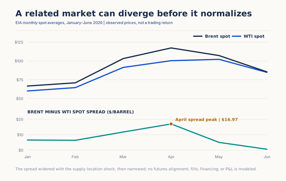
This is a selected relationship-break episode, not a pairs-trade return. A monthly average is known only after the month, the two spot series are not delivery-aligned futures, and the construction contains no formation window, hedge ratio, entry, fills, roll, financing, or costs. It therefore shows why a historical relationship may temporarily stop behaving like its old range—and why eventual narrowing does not prove that a live fade was executable.
Try it in Arizmic
Strategy composition
Build the premise with shipped signals
Use shipped relative-value signals to express and monitor a two-series spread, but keep economic pairing and cointegration validation outside the signal recipe. Entry requires a declared divergence; survival requires that the relationship has not visibly broken.
These are starting structures, not presets or evidence of an edge. Choose one, replace the bracketed decisions, and keep the signal roles separate as you test it.
Composition 01
Relative divergence with volatility and drawdown guards
Standardized-spread recipe- Relative DivergenceSpread and divergence state
- Volatility RegimeRelationship-risk state
- DrawdownStrategy-stop state
Data: OHLCV Bars, Aligned Secondary Series
View configuration and complete ruleHide recipe details
Composition 01
Relative divergence with volatility and drawdown guards
Relative Divergence
Spread and divergence state
Relative Divergence reports a benchmark-relative spread, its z-score, and rolling relationship diagnostics.
Configure
- window · [relationship window]
- Define the estimation history for spread normalization and rolling diagnostics.
Use the output
- zscore
- Create convergence candidates beyond [positive or negative threshold].
- close_beta
- Use the reported rolling beta as a monitored hedge-ratio input, not proof of cointegration.
- close_correlation
- Block or flag candidates when relationship strength falls below [minimum].
Volatility Regime
Relationship-risk state
Volatility Regime identifies periods when the spread’s previous normalization may no longer describe current movement.
Configure
- high_z_threshold · [high-volatility threshold]
- Define the state that blocks or reduces convergence exposure.
- low_z_threshold · [low-volatility threshold]
- Separate unusually quiet periods from normal conditions.
Use the output
- volatility_regime
- Apply [eligible regime policy] without using volatility as spread direction.
Drawdown
Strategy-stop state
Drawdown can enforce a portfolio-level pause when repeated divergence indicates that the relationship or execution assumptions may have failed.
Configure
No configurable parameter is required for this role.
Use the output
- drawdown
- Disable new entries or flatten at [declared strategy drawdown limit].
Assemble the rule
- Entry
- Enter the convergence side only after a completed-bar z-score extreme, sufficient relationship strength, and an eligible volatility state.
- Exit
- Exit at [z-score target], [timeout], [relationship-break rule], or [strategy drawdown limit].
- Decision time
- Estimate every rolling field from observations available through the decision bar and apply both legs on the next eligible event under declared fill assumptions.
- Sizing
- Use the declared beta or neutralization convention with gross and per-leg caps; do not infer hedge sizing from z-score alone.
Useful variations
- Compare a fixed formation-window beta with a rolling beta available at each decision time.
- Vary the relationship-strength gate separately from the z-score entry threshold.
- Report leg-level slippage and unhedged exposure when fills do not occur together.
Keep in view
Relative Divergence supplies rolling diagnostics, not a cointegration test or guarantee of convergence. A strategy using it must document the pair-selection and relationship-break logic separately.
Composition 02
Raw relative spread with distribution and risk context
Distribution-state recipe- Relative Close SpreadRaw spread observation
- Rolling DistributionEmpirical location
- EWMA VolatilityExposure scaler
Data: OHLCV Bars, Aligned Secondary Series
View configuration and complete ruleHide recipe details
Composition 02
Raw relative spread with distribution and risk context
Relative Close Spread
Raw spread observation
Relative Close Spread exposes the current close-to-benchmark relationship without embedding a trading threshold.
Configure
No configurable parameter is required for this role.
Use the output
- relative_close_spread
- Feed the observed spread into the declared rolling distribution and retain its raw value at entry.
Rolling Distribution
Empirical location
Rolling Distribution shows where the current series sits relative to its own recent median and quartiles.
Configure
- window · [distribution window]
- Define the reference sample used for location and percentile rank.
Use the output
- percentile_rank
- Create candidates outside [upper/lower percentile] rather than assuming a normal z-score.
- median
- Use return toward the rolling median as one declared exit variant.
EWMA Volatility
Exposure scaler
EWMA Volatility adjusts gross exposure when the relative series becomes more variable.
Configure
- lambda · [decay factor]
- Control how quickly risk reacts.
- return_kind · [return definition]
- Match the relative-series construction.
- annualization_bars · [bars per year]
- Match the actual interval.
- zscore_window · [volatility context]
- Use only for a separately declared volatility-state comparison.
Use the output
- ewma_volatility
- Scale gross pair exposure toward [risk target], subject to leg and leverage caps.
Assemble the rule
- Entry
- Enter convergence after the relative spread reaches the declared empirical tail and the pair remains eligible under its external relationship checks.
- Exit
- Exit at the rolling median, a less-extreme percentile, timeout, or relationship invalidation.
- Decision time
- Freeze the decision-bar percentile and spread; any rolling median exit remains a live signal and must be modeled that way.
- Sizing
- Use capped inverse-volatility gross exposure and the separately declared leg-neutralization rule.
Useful variations
- Compare empirical-percentile and z-score entries on identical dates.
- Freeze the exit reference at entry versus allow the rolling median to update.
- Use formation/trading splits so percentile history is not fit with future observations.
Keep in view
A rolling distribution can adapt to a broken relationship and make a widening spread look statistically ordinary. External economic and stability checks remain necessary.
Ask the AI Companion
Draft this strategy
Turn a relationship between two assets into a simple pairs-trading draft without hiding the assumptions behind the spread.
I want to create a pairs-trading strategy for [asset A] and [asset B] because [brief reason they should be related]. Recommend how their relationship should be measured, how much historical data and which trading timeframe I should start with, and a sensible way to size the two legs. Then build a strategy that seeks to profit from unusually large divergences while stopping when the relationship appears to have materially changed.
Extend it in Marimo
Begin from a retained two-series Study so pair choice, formation history, and candidate dates remain traceable.
Track whether divergence signals remain connected to a stable relationship across formation and trading windows.
- Bring in
- engine-reported relative spread, z-score, beta, correlation, volatility state, drawdown, decisions, and fills, declared formation and trading windows, leg-level prices, quantities, costs, and retained candidate identifiers
- Build
- formation-versus-trading spread and parameter panels, relationship-drift timeline with candidate and exit markers, leg-level P&L, slippage, and unhedged-exposure reconciliation
Interpretation: A widening spread is not automatically a better entry. Treat beta drift, collapsing correlation, changing variance, or repeated timeouts as evidence that the convergence story may no longer apply.
Value origin: Signal outputs, decisions, fills, costs, and retained metrics are engine-reported. Formation/trading comparisons, drift flags, and custom leg-reconciliation summaries are notebook-derived.
With Companion: Ask Companion to draft relationship-drift and leg-reconciliation cells, inspect the point-in-time windows, then explicitly apply the reviewed diff.
Further reading
- Engle and Granger, “Co-Integration and Error Correction: Representation, Estimation, and Testing” (1987) — Establishes the cointegration and error-correction framework; passing a historical test does not make a particular economic relationship permanent.
- Gatev, Goetzmann, and Rouwenhorst, “Pairs Trading: Performance of a Relative-Value Arbitrage Rule” (2006) — Tests a transparent distance-based US-equity design with separate formation and trading periods from 1962–2002; it is not a cointegration strategy.
- Do and Faff, “Does Simple Pairs Trading Still Work?” (2010) — Reassesses simple pairs trading and reports declining profitability alongside stronger performance during prolonged turbulence, illustrating both decay and regime dependence.
- Avellaneda and Lee, “Statistical Arbitrage in the US Equities Market” (2010) — Constructs mean-reverting residuals using PCA and sector ETFs and documents substantial deterioration after 2002; it represents broader residual arbitrage rather than a simple two-stock pair.
- US Energy Information Administration, monthly WTI spot prices and monthly Brent spot prices — Supply the official monthly averages used in the selected 2026 chart; they are spot benchmarks, not synchronized or executable futures legs.
- US Energy Information Administration, “Crude oil and petroleum product prices increased sharply in the first quarter of 2026” and “Petroleum markets responded to disruptions in the Middle East in the second quarter” — Explain the disruption-driven widening and subsequent change in crude-market conditions; neither constitutes a pairs-trade backtest.