Mean reversion asks whether a displacement is temporary
Mean reversion is the hypothesis that a measured variable tends to move back toward a reference after moving unusually far away. The variable might be a price, a return, a yield spread, or the residual between two related assets. The reference might be a rolling average, a session VWAP, or an estimated economic relationship.
The reference is the anchor. Without naming it, “price should come back” has no testable meaning. Back to yesterday’s close, a 20-day average, and a cointegrating spread are three different claims.
Mean reversion also needs a horizon. Price can revert around an intraday VWAP while remaining in a year-long uptrend. Momentum and reversion are therefore not universal opposites. They conflict only when they describe the same variable over the same interval.
Most importantly, an anchor is not automatically fair value. It is a summary of past information whose continued relevance must be tested.
Why a displacement might close
Temporary buying or selling pressure can move price farther than the available liquidity can immediately absorb. Dealer inventory, mechanical rebalancing, forced liquidation, and short-lived attention can all create an imbalance that fades once the urgent flow is complete.
Some variables also have stronger economic constraints. Related contracts may be linked through conversion, financing, or substitution; a portfolio residual may fluctuate around a stable exposure relation. In those cases the anchor has more substance than an arbitrary chart average, although transaction costs and structural change can still prevent convergence.
The competing explanation is repricing. New information may make the old reference obsolete. A reversion rule is consequently short the persistence of the displacement: it often wins small amounts when ordinary noise closes, then loses much more when the move marks a genuine regime change.
The anatomy of a reversion rule
| Decision | Common choices | What the choice means |
|---|---|---|
| Variable | Price, return, spread, residual | Defines what is expected to revert |
| Anchor | Rolling mean, VWAP, prior value, fitted relation | Defines “back” |
| Distance | Raw units, percentage, volatility units, z-score | Determines what counts as unusual |
| Entry | Immediate extreme, close beyond band, or return inside band | Trades early entry against reversal confirmation |
| Target | Anchor, inner band, fixed reward, or time exit | Defines success |
| Invalidation | Stop, timeout, volatility state, structural break | Defines evidence that the anchor failed |
| Exposure | Fixed, risk-scaled, or capped averaging | Determines how a prolonged deviation affects capital |
A z-score does not solve these decisions. It simply expresses the current distance in units of an estimated standard deviation. If the average and standard deviation are unstable, the score is unstable too.
A simple example
Illustrative example. Assume a completed daily observation gives:
- rolling anchor: 100;
- estimated standard deviation of the displacement: 2; and
- current price: 95.
The normalized displacement is . A predeclared long reversion rule might enter at the next eligible event when the score is below −2, target the inner band at −0.5, and invalidate after five days or below −4.
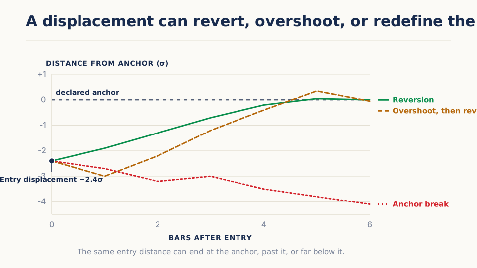
Three paths show why the definition matters:
- Price rises to 99 while the anchor stays near 100. The displacement closes as hypothesized.
- Price remains at 95 while the rolling anchor falls to 97. The score improves, but little economic recovery occurred; the moving anchor partly chased the loss.
- Price falls to 90 after material news. The old anchor no longer describes the state, and a rule without invalidation keeps increasing its exposure to a broken thesis.
The second case is why researchers should inspect both normalized distance and the raw path. A prettier z-score is not necessarily a profitable reversion.
Why the two sides are not mirror images
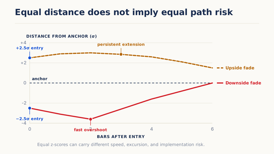
A score of −2.5 and a score of +2.5 are equally far from the anchor mathematically. They do not create equal trades economically.
For an equity index, long-run positive drift can make an upside extension persist while a short reversion position pays financing, borrow, and opportunity costs. Downside moves often arrive faster, with larger volatility and thinner liquidity, so buying the lower extension can experience a deeper overshoot before any rebound. Those are different risks: persistence asks how long a deviation lasts, while excursion asks how far it travels before closing.
Empirical findings are conditional. Some US index samples have shown quicker and larger reversal after negative monthly returns, while broad-index evidence also shows unequal waiting times for matched gains and losses. Those findings motivate side-specific tests; they do not establish a universal rule for individual stocks, futures, intraday bars, or a different sample.
The practical response is to design two sleeves rather than force one symmetric rule:
| Design choice | Downside fade | Upside fade |
|---|---|---|
| Position | Buy an unusually low observation | Short an unusually high observation |
| Important baseline | Long-only exposure over the same holding window | Flat or hedged exposure that does not inherit positive drift |
| Main path risk | Fast volatility expansion and an overshoot below the entry band | A persistent rally that keeps the short away from its target |
| Implementation burden | Gap, spread, and capital required during the selloff | Borrow, financing, squeeze risk, and short-sale constraints |
| Useful invalidation | Volatility or structural-break state, hard distance, timeout | Trend persistence, borrow change, hard distance, timeout |
| Report separately | Adverse excursion and time to rebound | Time in trade and distance traveled before reversion |
Illustrative example. Keep the anchor fixed at 100 and the estimated dispersion at 2 for one decision:
| Completed observation | Normalized distance | Candidate next-event action | Inner target | Hard invalidation |
|---|---|---|---|---|
| 95 | −2.5 | Long the downside sleeve | −0.5 | −4.0 |
| 105 | +2.5 | Short the upside sleeve | +0.5 | +4.0 |
The thresholds are symmetric only so the comparison is readable. The study should still allow different timeouts, risk caps, and eligibility filters. If volatility and the anchor update after entry, preserve both the entry-time distance and the live distance; otherwise a moving denominator can make one side appear to improve without price moving toward the original reference.
What a credible result would look like
Credibility comes from a stable relationship among choices. Wider entry bands should normally create fewer, more extreme opportunities. Longer timeouts should change both convergence rate and capital usage. Costs should matter more at shorter horizons.
A result becomes difficult to trust when the anchor continuously moves toward losing trades, when most “profits” remain unrealized at the test boundary, or when one threshold produces an isolated success. The rule should also be tested around known structural changes rather than only during calm, range-bound periods.
Failure modes are part of the strategy
- Broken anchor: new information or a regime shift makes the reference irrelevant.
- Asymmetric tail: many small wins are overwhelmed by a few persistent moves.
- Scale instability: volatility expands, so a formerly extreme raw distance becomes ordinary—or the reverse.
- Overlapping observations: frequent signals can represent one prolonged event rather than independent opportunities.
- Cost sensitivity: small expected reversions vanish after spread, impact, and missed fills.
- Averaging down: adding exposure as price moves farther away can hide risk until a capital limit is reached.
Try it in Arizmic
Strategy composition
Build the premise with shipped signals
Define a measurable displacement, enter only when the surrounding state does not already look like strong continuation, and state in advance what counts as reversion, timeout, or anchor failure.
These are starting structures, not presets or evidence of an edge. Choose one, replace the bracketed decisions, and keep the signal roles separate as you test it.
Composition 01
Standardized displacement with trend exclusion
Oscillator recipe- Oscillator RegimeDisplacement state
- ADX/DMIContinuation-risk gate
- Wilder ATRRisk and overshoot scale
Data: OHLCV Bars
View configuration and complete ruleHide recipe details
Composition 01
Standardized displacement with trend exclusion
Oscillator Regime
Displacement state
Oscillator Regime standardizes price relative to its recent distribution and labels lower, neutral, and upper states.
Configure
- window · [normalization window]
- Define the history used to judge whether displacement is unusual.
- lower_threshold · [lower entry threshold]
- Define a candidate oversold state before observing the outcome.
- upper_threshold · [upper entry threshold]
- Define a candidate overbought state symmetrically or document the asymmetry.
Use the output
- zscore
- Use the signed z-score to measure entry distance and progress back toward the center.
- regime
- Create a candidate only in the declared lower or upper regime.
ADX/DMI
Continuation-risk gate
ADX/DMI helps distinguish a stretched range from a strongly directional move that may keep extending.
Configure
- window · [trend-strength window]
- Measure continuation risk over the intended holding horizon.
Use the output
- adx
- Block or reduce new reversion entries above [maximum trend strength].
- plus_di
- For a short reversion, flag strong positive directional pressure.
- minus_di
- For a long reversion, flag strong negative directional pressure.
Wilder ATR
Risk and overshoot scale
ATR turns raw displacement and protection distances into current-volatility units.
Configure
- window · [ATR window]
- Estimate the scale of plausible overshoot.
Use the output
- atr
- Set [entry or invalidation distance] and position size in ATR units.
Assemble the rule
- Entry
- After a completed bar enters the lower or upper oscillator regime, take the opposite-direction candidate only if ADX/DMI pass the continuation-risk policy.
- Exit
- Exit at [z-score center/partial reversion], [timeout], or [ATR-based anchor failure], whichever occurs first.
- Decision time
- Do not backdate the entry to the intrabar extreme; decide only after the threshold state is known.
- Sizing
- Scale units to the ATR-based invalidation distance under a fixed risk budget.
Useful variations
- Compare center exit with a partial-reversion target while keeping entry fixed.
- Treat high ADX as a hard block versus reduced size.
- Partition outcomes by initial z-score distance and time to reversion.
Keep in view
A standardized extreme can become more extreme when the underlying regime changes. The trend gate reduces some continuation exposure but cannot prove that the anchor is still valid.
Composition 02
Band location with reversal confirmation
Band-state recipe- Bollinger Band PositionRelative location
- ROCReversal confirmation
- Volatility RegimeState policy
Data: OHLCV Bars
View configuration and complete ruleHide recipe details
Composition 02
Band location with reversal confirmation
Bollinger Band Position
Relative location
Band Position expresses where price sits relative to a rolling mean and standard-deviation envelope.
Configure
- window · [band window]
- Define the local anchor and dispersion history.
- std_multiplier · [band width]
- Set how far price must travel before it becomes a candidate.
Use the output
- position
- Create a candidate below [lower position] or above [upper position].
ROC
Reversal confirmation
Short-horizon ROC can require the displacement to stop extending before entry rather than buying or selling the first touch.
Configure
- window · [reversal lookback]
- Use a shorter horizon than the band anchor to detect a change in direction.
Use the output
- roc
- For a long, require ROC to recover above [threshold]; reverse the condition for a short.
Volatility Regime
State policy
Volatility Regime separates an ordinary band excursion from a volatility shock where the same threshold may have a different meaning.
Configure
- high_z_threshold · [high-volatility threshold]
- Define the state that blocks or reduces exposure.
- low_z_threshold · [low-volatility threshold]
- Define the low-volatility state used in comparison.
Use the output
- volatility_regime
- Apply a declared eligible-state policy without treating volatility as direction.
Assemble the rule
- Entry
- Enter only after an extreme band position, a completed-bar ROC reversal, and an eligible volatility state coincide.
- Exit
- Exit at [middle-band/position target], an opposite displacement, timeout, or invalidation.
- Decision time
- The reversal confirmation delays entry; the original band touch is context, not the trade timestamp.
- Sizing
- Use [fixed risk or separate volatility sizing] consistently across regime variants.
Useful variations
- Compare first-touch entry with confirmed-reversal entry and report the missed and delayed trades.
- Use middle-band exit versus zero band-position exit.
- Keep thresholds fixed while comparing normal and high-volatility states.
Keep in view
Confirmation can make the historical entry look cleaner by waiting for recovery. Measure the price paid for that information and do not score the trade from the earlier extreme.
Ask the AI Companion
Draft this strategy
Turn the guide’s mean-reversion idea into a simple draft while explaining the anchor and the risk that it may stop being useful.
I want to create a mean-reversion strategy for [instrument] that detects when price has moved unusually far from a meaningful reference and seeks to profit when that displacement closes. Recommend the reference, timeframe, and holding horizon you would use as a starting point, including whether upward and downward extensions should be treated differently for this instrument. Then build the strategy for me and explain how it will recognize when the reference is no longer reliable.
Extend it in Marimo
Begin from a retained Study so entry thresholds, exits, and anchor-failure definitions stay connected to their candidates.
Trace every displacement from candidate through confirmation, reversion, overshoot, timeout, or invalidation.
- Bring in
- engine-reported displacement, regime, ADX/DMI, ATR, decisions, and fills, declared anchor, thresholds, exits, and timeouts, retained trades, costs, and candidate identifiers
- Build
- event-aligned displacement paths from the actual decision time, time-to-reversion and maximum-adverse-excursion distributions, outcome table by entry distance, trend strength, and volatility state
Interpretation: A high eventual reversion rate can still be unusable if overshoot, holding time, or anchor failure grows faster than the expected convergence.
Value origin: Signal values, decisions, fills, and retained outcomes are engine-reported. Event alignment, time-to-reversion labels, and custom overshoot partitions are notebook-derived.
With Companion: Ask Companion to draft a path-analysis cell set, preview the diff, inspect the event definitions and time alignment, then apply it explicitly.
Further reading
- Poterba and Summers, “Mean Reversion in Stock Prices: Evidence and Implications” (1988) — Finds point estimates consistent with short-horizon continuation and longer-horizon reversal across US and international markets, while emphasizing that low-powered conventional tests cannot reject a random walk.
- Kim, Nelson, and Startz, “Mean Reversion in Stock Prices? A Reappraisal of the Empirical Evidence” (1991) — Re-examines the long-horizon result using randomization and prewar/postwar splits, finding weaker evidence that is concentrated before World War II.
- Mukherji, “Are Stock Returns Still Mean-Reverting?” (2011) — Uses block-bootstrap tests through 2007 and finds that long-horizon reversion weakened in later decades and varies by company size and holding period.
- Nam, Pyun, and Avard, “Asymmetric Reverting Behavior of Short-Horizon Stock Returns: An Evidence of Stock Market Overreaction” (2001) — Finds quicker and larger reversal after negative monthly returns in value-weighted US indexes from 1926–1997; the result is specific to that sample and nonlinear model.
- Jensen, Johansen, and Simonsen, “Inverse Statistics in Economics: The Gain–Loss Asymmetry” (2003) — Measures unequal waiting times for matched gains and losses, supporting separate analysis of path direction and duration rather than establishing a profitable fade rule.
- Nagel, “Evaporating Liquidity” (2012) — Interprets short-term equity reversal returns as compensation for liquidity provision and shows that this compensation rises during market turmoil.