A large order creates a timing problem
Imagine that you need to buy a large block of shares before the end of the day. Buying them all at once is quick, but your own demand may push up the price you pay. Spreading the order across several hours is gentler, but it gives the market more time to move before you finish.
Execution scheduling is the choice between those two pressures. Trade faster and the order may become more expensive. Trade more patiently and a larger part of it remains exposed to whatever the market does next.
There is no single pace that suits every order. Exiting a position that has become too risky may be worth doing quickly, even at a higher cost. Building a position from a slow-moving signal may allow more patience.
Where Almgren–Chriss fits
Almgren–Chriss gives this timing choice a mathematical shape. You give the model the size of the order, the time available, a view of trading costs and market volume, and an estimate of how much the price tends to move. You also choose how much weight to place on the uncertainty created by waiting.
The result is a schedule showing how much to trade in each interval. One schedule might divide the order evenly. Another might trade a large amount at the beginning and gradually slow down.
The same schedule can be drawn as the amount still left to trade after each interval. This is called the inventory path. A straight decline means equal trades. A steep drop near the beginning means the order is front-loaded.
The setting that controls how much weight the model gives to waiting is called risk aversion. Here, it works like an urgency dial: turn it up and more of the order is traded early; turn it down and the order is spread more evenly through time.
Two forces pull the schedule in opposite directions
The first force is the cost of trading a large amount at once. The share of market volume represented by your trade is known as participation. As participation rises, the order is more likely to reach beyond the best available prices. Almgren–Chriss represents that extra execution cost as temporary impact.
The second force is the uncertainty created by waiting. Any shares left to buy may later be cheaper, but they may also be more expensive. Volatility gives the model an estimate of how wide those price moves could be. The more shares still waiting—and the longer they wait—the wider the range of possible final costs.
Almgren–Chriss looks for a balance between these forces. Patience can reduce expected impact. Urgency can reduce the uncertainty around the eventual cost.
Three ways to trade the same order
Illustrative example. Suppose 100,000 shares must be bought over five equal intervals, with 500,000 shares of market volume in each one. Assume crossing the spread adds $0.01 per share, price volatility is $0.10 per share in each interval, and temporary impact rises with participation.
Keeping those conditions and the deadline unchanged, compare three settings of the urgency dial:
| Schedule | What it favors | Trades, intervals 1 → 5 | Expected modeled cost | Cost uncertainty (standard deviation) |
|---|---|---|---|---|
| Patient | Lowest expected cost | 20,000 · 20,000 · 20,000 · 20,000 · 20,000 | $2,000 | $10,954 |
| Balanced | A middle ground | 39,775 · 24,718 · 15,842 · 10,925 · 8,740 | $2,320 | $7,315 |
| Urgent | Less uncertainty from waiting | 61,818 · 23,636 · 9,091 · 3,637 · 1,818 | $3,240 | $4,126 |
The share amounts are rounded for display. Expected cost includes the $1,000 spread cost and the model's estimate of temporary impact. The final column shows how widely the total cost could vary while part of the order remains exposed to price movement.
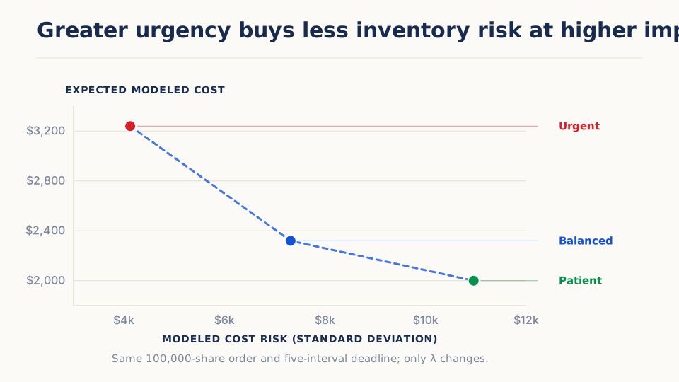
The patient schedule buys 20% in every interval. It has the lowest expected cost, but it leaves more of the order waiting for longer. The urgent schedule buys about 62% immediately. Its expected cost is higher, but its range of possible costs is much narrower. The balanced schedule sits between them.
This is the central idea of the model: reducing uncertainty has a price. The best choice depends on how valuable earlier completion is for that particular order.
The comparison is fair because the order size, deadline, market volume, spread, impact, and volatility stay the same. Only urgency changes. If one schedule had five minutes to finish and another had all day, they would no longer be solving the same problem.
To keep the example focused, it leaves out price drift, changing volume, persistent impact, additional fees, incomplete fills, and signal decay. Those features matter in a real execution problem, but they are not needed to see the basic trade-off.
What changes the shape of the schedule
Once the two forces are clear, the direction of the model becomes intuitive:
| When this rises | The schedule tends to | Why |
|---|---|---|
| Urgency setting | Trade more of the order early | Waiting receives a larger penalty |
| Price volatility | Trade more of the order early | The unfilled amount is exposed to wider price moves |
| Cost of trading large slices | Spread the order out | Concentrated trading becomes more expensive |
| Market volume | Trade more of the order early, all else equal | The same trade becomes a smaller share of the market |
These are tendencies, not fixed rules. Minimum trade sizes, participation limits, changing volume, venue restrictions, and incomplete fills can all reshape what is actually possible.
What “optimal” really means
In Almgren–Chriss, optimal means best for the assumptions supplied to the model. If expected volume is too high or impact is underestimated, the model can produce a precise schedule for a poor description of the market.
The benchmark matters too. Measuring cost from the moment the decision was made can tell a different story from measuring it from market arrival or the closing price. So can changing the deadline, the impact estimate, or the value placed on finishing early.
The urgency setting deserves an economic reason: perhaps a liquidation deadline, a fast-decaying signal, or a risk limit. Choosing it after seeing which historical price path makes the schedule look best defeats the purpose of the model.
How Almgren–Chriss differs from simpler schedules
Almgren–Chriss is not simply a more elaborate name for TWAP or POV. Each method responds to a different part of the problem:
| Method | How it trades | What makes it change | Main trade-off |
|---|---|---|---|
| Immediate | Trades the full amount now | Nothing | Finishes quickly but may consume substantial liquidity |
| TWAP | Divides the order across a time grid | The clock | Simple and predictable, but usually ignores current volume |
| POV | Trades a chosen share of observed market volume | Realized volume | Adapts to activity, but low volume can delay completion |
| Forecast-volume schedule | Follows a volume pattern estimated in advance | The expected volume profile | Can match the trading day, but depends on the forecast |
| Almgren–Chriss | Shapes the schedule around impact, volatility, urgency, and a deadline | Its assumptions and constraints | Makes the cost-versus-uncertainty choice explicit |
POV means percentage of volume or participation of volume. It is different from Point of Control in a volume profile. A forecast-volume schedule is also different from using volume-weighted average price (VWAP) as an execution benchmark or a trading signal.
When volume is constant and no weight is placed on uncertainty from waiting, the simplest Almgren–Chriss schedule divides the order into equal time slices. In that special case, it has the same shape as TWAP. Changing volume, adding constraints, or using a different impact model breaks that equivalence.
A model should earn its complexity
The right comparison is not Almgren–Chriss against nothing. Put it beside immediate execution, TWAP, POV, and a forecast-volume schedule, then give every method the same order, deadline, benchmark, fees, spread, and market paths.
Average cost is only part of the result. A useful comparison also shows how often the order finishes, how long completion takes, how much is left behind, how widely costs vary, and what happens during adverse outcomes. It should also show whether the conclusion survives reasonable changes to the volume, volatility, and impact estimates.
A comparison becomes misleading if a volume schedule uses information that was not available at the time, or if a method appears cheap only because it leaves the hardest quantity unfilled. In either case, the apparent improvement comes from changing the problem rather than solving it better.
The hard part is estimating the inputs
An optimizer can return a schedule to many decimal places while the impact estimate behind it remains uncertain. Impact varies across instruments, venues, order types, times of day, participation levels, and market conditions. An estimate taken from calm trading in one instrument may say little about a larger order during a volatile session.
Small changes to reasonable inputs should not completely reshape the first trade. If they do, the schedule is fragile and should be treated as a range of possibilities rather than a single answer.
Price volatility is also different from signal decay. A position built from a short-lived signal may need to be completed quickly even when ordinary price variance looks modest. A slow-moving portfolio adjustment may not deserve the same urgency.
Finally, the market will not hold still for the model. Volume, spreads, depth, and volatility can change during the order, while participation limits, lot sizes, venue rules, and fill behavior can make the smooth mathematical path impossible to follow exactly.
Optional: the mathematics behind the schedule
The sections above are enough to understand the model's practical meaning. What follows expresses the same trade-off in notation for readers who want to see how the schedule is calculated.
The objective function
In the simplified model, the preferred path has the lowest combination of expected implementation cost and cost uncertainty:
is implementation cost in dollars relative to the chosen benchmark. is its expected value, and is its variance in dollars squared. The parameter has units of inverse dollars and says how much weight to place on that variance. A larger gives uncertainty from waiting more influence and produces a more urgent schedule.
A numerical value of is not portable across currencies, order sizes, horizons, volatility conventions, or differently normalized objectives.
Describing the inventory path
Let be the number of shares to complete over equal intervals. Let be the shares remaining after interval , and let be the shares traded during that interval:
The sequence is the inventory path. A straight decline means equal trades; a steep early decline means a front-loaded schedule.
For the illustrative model, assume each interval has shares of market volume, the paid half-spread is dollars per share, and temporary impact per share is dollars times the trade's participation rate. Expected modeled cost is:
The spread term is fixed once is fixed. The squared trade-size term makes concentrated trading progressively more expensive and therefore rewards patience.
Now assume independent, zero-mean price changes with standard deviation dollars per share in each interval. The cost variance is:
Shares carried later appear in more uncertain intervals, so this term rewards urgency. The final inventory is zero and adds nothing to the sum.
The original framework also includes permanent impact. Under the simplest linear permanent-impact assumption and a fixed order size, most of that contribution is common across schedules; depending on the discrete-time convention, it can also adjust the effective quadratic-impact coefficient. Temporary impact versus remaining-inventory risk is the essential scheduling mechanism.
The closed-form path in the simple case
With constant volume and volatility and linear temporary impact, the remaining inventory has this shape:
is a dimensionless curvature parameter determined by urgency, volatility, volume, and temporary impact. The expression is useful for its direction rather than for memorization:
- when , the limiting path is straight and the trades are equal;
- increasing or front-loads the schedule;
- increasing makes large early trades more expensive and favors patience; and
- increasing lowers participation for a given trade and makes urgency less costly in this stylized model.
In the earlier example, shares, , and shares. The half-spread is 0.01 dollar per share, the temporary-impact coefficient is 0.25 dollars per share, and the interval volatility is 0.10 dollars per share. The patient, balanced, and urgent paths use values of , , and per dollar, respectively. Those values reproduce the three displayed schedules; they are illustrative settings, not recommended defaults.
Further reading
- Almgren and Chriss, “Optimal Execution of Portfolio Transactions” (2001) — Derives the expected-cost and cost-variance frontier under explicit temporary- and permanent-impact assumptions. It is the canonical baseline, not a ready-made schedule for every market.
- Perold, “The Implementation Shortfall: Paper Versus Reality” (1988) — Defines the decision-price benchmark and accounts for both completed executions and missed trades. It establishes what an execution schedule should be measured against.
- Bertsimas and Lo, “Optimal Control of Execution Costs” (1998) — Develops dynamic execution policies in a stochastic-control setting. It is useful for seeing how conditioning decisions on evolving information differs from committing to one static schedule.
- Almgren, “Optimal Execution with Nonlinear Impact Functions and Trading-Enhanced Risk” (2003) — Extends optimal liquidation to nonlinear impact and additional execution-related uncertainty. It demonstrates how strongly the recommended trajectory depends on the assumed impact function.
- Almgren, Thum, Hauptmann, and Li, “Direct Estimation of Equity Market Impact” (2005) — Estimates temporary and permanent impact from institutional equity orders. It provides empirical context for why calibration, participation, and trade-duration assumptions matter.
- Gatheral and Schied, “Dynamical Models of Market Impact and Algorithms for Order Execution” (2013) — Reviews transient and dynamic impact models, optimal-execution stability, and conditions associated with price manipulation. It is model-risk context rather than an implementation recipe.